Hooke’s law in one sentence
Within its proportional range, a spring’s extension is proportional to the force applied to it: F = kx. Here x is the change in length from the unloaded length, not the total length, and k is the spring constant. If F is in newtons and x is in metres, k is in newtons per metre (N/m). A larger k means a stiffer spring: the same load produces less extension.
This F is the magnitude of the applied force needed to hold the spring at a particular extension. The force exerted by the spring points the other way and is written Fspring = −kx when x is a signed displacement from its unstretched position. The minus sign describes direction; it does not make the spring constant negative.
Extension is not the spring’s total length
Measure the unloaded length L₀ first. If the loaded length is L, extension is x = L − L₀. For example, a spring that grows from 0.30 m to 0.35 m has extended by 0.05 m, not 0.35 m. If the question gives centimetres, convert the extension to metres before using a k stated in N/m.
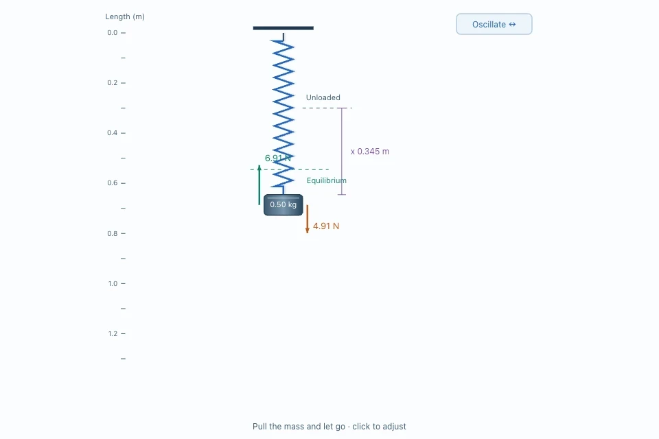
For a mass hanging still from an ideal vertical spring, the downward weight mg balances the upward spring force. Therefore mg = kx at static equilibrium. During a pull-and-release oscillation the forces are usually unbalanced, so mg = kx should not be applied to every moving frame.
Worked example: find k from a hanging mass
Suppose a 0.20 kg mass hangs at rest and lengthens a spring by 4.0 cm. Use g = 9.81 m/s². The load is F = mg = 0.20 × 9.81 = 1.962 N, and the extension is 0.040 m. So k = F/x = 1.962/0.040 = 49.05 N/m, or about 49 N/m to two significant figures.
A useful check is to predict a second static reading. At the same gravity and with the same spring, a 0.40 kg mass should give about 0.080 m extension while the spring stays in its proportional range. It will not have a total length of 0.080 m: add the unloaded length to obtain that.
Read the slope of a force–extension graph
Plot applied force F on the vertical axis and extension x on the horizontal axis. In the straight-line region, gradient ΔF/Δx equals k. For example, if force rises from 1.0 N to 3.0 N while extension rises from 0.020 m to 0.060 m, the gradient is 2.0/0.040 = 50 N/m. Use two well-separated points on a best-fit line rather than a single noisy pair.
Some classes put extension on the vertical axis instead. That gradient is Δx/ΔF = 1/k, so inspect the axes before naming the slope. An apparent intercept can signal a zero offset or method problem. A curved region means one constant k no longer describes all those points; do not extend a straight-line fit beyond the data that support it.
Elastic energy is the area under the graph
For an ideal linear spring stretched from zero to x, stored elastic potential energy is E = ½kx². It also equals the triangular area under a graph of applied force against extension: E = ½Fx. Using k = 50 N/m and x = 0.040 m gives E = ½ × 50 × 0.040² = 0.040 J.
The factor ½ matters because force rises from zero to kx as the spring stretches. Multiplying the final force by the full extension would double the answer. During ideal undamped oscillation, energy changes between motion and stored energy; the spring’s elastic energy alone is not constant.
Try a force–extension investigation
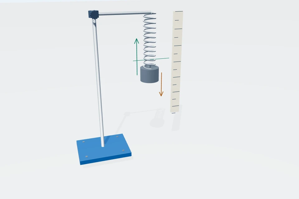
Open the 3D Hooke’s law lab and choose “Measure · static equilibrium.” Keep spring stiffness and gravity fixed. Record the unloaded length, then use several hanging masses, including 0.20 kg and 0.40 kg if the chosen stiffness keeps both extensions within the model’s range. For each trial, calculate load as mg and extension as loaded length minus unloaded length. Plot force against extension and estimate k from its slope before checking the displayed spring stiffness.
Then choose “Oscillate · pull and release,” set a nonzero release displacement and compare no damping with a positive damping ratio. The 3D mass can be pulled directly. Watch the mass pass through equilibrium: it still has speed there, even though the upward spring force equals the weight at that instant. The 2D view can make the force arrows and graph easier to inspect.
Where the model stops applying
A real spring has a finite range over which force and extension are proportional. The limit of proportionality marks the end of the straight-line relationship; the elastic limit concerns whether it returns to its original length after unloading. They are different ideas. Real springs can also have mass, friction and permanent deformation.
Labmora deliberately uses an ideal linear spring and does not model plastic deformation or compression. Its “spring stiffness” setting fixes k, so the model’s straight line should not be presented as evidence that every real spring stays linear at large loads. Use actual apparatus to investigate limits and uncertainty.
Sources and further reading
- OpenStax College Physics: Hooke’s law and force–displacement graphs
- OpenStax University Physics: elastic potential energy
Found an error or a confusing explanation? Send a science correction.